
General Usage
What does Flint do?
Flint provides you with a Framework to create and manipulate Tensors. Tensors are just multidimensional data arrays with the same shape along each dimension.
A Vector or a Matrix are Tensors too. You can create a 6-dimensional Tensor with the shape of 256, 128, 64, 32, 1024, 53 (here shape is always denoted from inner to outer, so 256 is the outer most dimension).
The great thing about Flint: you can apply operations to those Tensor, for example addition, multiplication, you can convolve Tensor, do Matrix multiplication and so on.
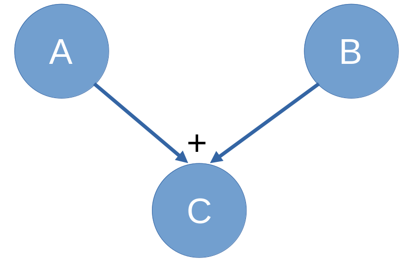
Flint is then able to execute those operations, which are stored in an operational graph.
(a graph were each node either represents a data node (so it stores data you calculated or put there) or a operation itself, that has been executed or still has to be executed. Those nodes can be connected in a graph: e.g. if you sum up to nodes A and B to the result C, the node C is the child of its parents A and B).
Allthough if you use the C++ frontend you won't get in touch too much with this graph it enables efficient gradient calculation which is the core functionality for machine learning in a Tensor Execution framework. You can execute these Tensor on your CPU or on a OpenCL capable device like a GPU, for more see the Execution section.
Flint provides an automatic memory management system for your Tensors and all their allocated data with reference counting in the graph, for more see the Data section.
The great thing about Flint: you can apply operations to those Tensor, for example addition, multiplication, you can convolve Tensor, do Matrix multiplication and so on.
Flint is then able to execute those operations, which are stored in an operational graph.
(a graph were each node either represents a data node (so it stores data you calculated or put there) or a operation itself, that has been executed or still has to be executed. Those nodes can be connected in a graph: e.g. if you sum up to nodes A and B to the result C, the node C is the child of its parents A and B).
Allthough if you use the C++ frontend you won't get in touch too much with this graph it enables efficient gradient calculation which is the core functionality for machine learning in a Tensor Execution framework. You can execute these Tensor on your CPU or on a OpenCL capable device like a GPU, for more see the Execution section.
Flint provides an automatic memory management system for your Tensors and all their allocated data with reference counting in the graph, for more see the Data section.
Execution of Tensors
There are two different backends for the execution of Operations with two different execution strategies.
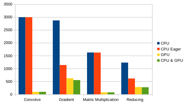
Benchmarks of example programs on an Intel i5 10600K and an AMD Radeon 5700XT,
time in milliseconds As one can see from the benchmarks especially for many small operations eager execution is better for the CPU backend since the performance load is better distributed and it has much less overhead. For the GPU backend lazy execution is far better. The best overall performance is achieved with activating both backends without eager execution, where Flint chooses one by some heuristics. This yields currently a few milliseconds, but with some additional optimizations i am working on it might be much more.
- Lazy Execution: the nodes are only executed if the operation enforces it (e.g. matrix multiplication or reduction enforces complete execution of the parental nodes)
or `fExecuteGraph` (in C) or `.execute()` (in C++) is called.
Else the graph is constructed with the operations, but the result data is only calculated for a node if it is executed.
- CPU Backend
A simple thread pool that is initialized with as many threads as your CPU supports. The calculation of a operation may be split into multiple work packages that are then distributed to the threads.
In the case that parental nodes don't have result data yet, those are executed first (i.e. the unexecuted parental subtree of the node is executed sequentially in its topological order).
Fast for small Tensors or lightweight operations since the overhead is little. - OpenCL Backend
Constructs a OpenCL kernel for the complete unexecuted graph and executes it (has a cache to lookup and store already compiled kernels). This allows implicit execution of only those parts of the parental data of a node that are actually important for the last node. E.g.Tensor<float, 3> m1 = Tensor<float, 3>::constant(3.141592, 128, 128, 128); Tensor<float, 3> m2 = Tensor<float, 3>::constant(42.0007, 128, 128, 128); Tensor<float, 3> m3 = m1.matmul(m2).slice(TensorRange(0, 4), TensorRange(0, 4), TensorRange(0, 2)); m3.execute();
Here it is possible for the GPU Backend to lazily only compute the 4*4*2 elements of m3 and their corresponding elements in the Matrix multiplication without having to calculate the other 2097120 elements (128*128*128 = 2097152 elements).
- CPU Backend
-
Eager Execution: Each node has to be executed during construction. The OpenCL backend then resorts to the generation of general operation kernels for each operation
(one program per operation, one kernel per possible datatype combination of the parameters).
This reduces the overhead of the CPU Backend alot but interferes alot with OpenCL optimizations.
Benchmarks of example programs on an Intel i5 10600K and an AMD Radeon 5700XT,
time in milliseconds As one can see from the benchmarks especially for many small operations eager execution is better for the CPU backend since the performance load is better distributed and it has much less overhead. For the GPU backend lazy execution is far better. The best overall performance is achieved with activating both backends without eager execution, where Flint chooses one by some heuristics. This yields currently a few milliseconds, but with some additional optimizations i am working on it might be much more.
Data Management and Initialization
Flint needs to be initialized and cleaned up. Initialization can be done implicitly (when no backend had been initialized during a call to an execution method the corresponding or both backends will be initialized). It is possible to initialize only one of the two backends or both in which case Flint is allowed to choose one in the execute call.
When you are done using Flint, the backends need the oportunity to shut down started threads and free memory. Use the cleanup Method for that. In C any memory needed to store the Tensors is allocated by the framework itself. Additionally to allow function calls like
reference counting is used in the nodes to keep track which node is still used. Freeing one node tries to free its predecessors too if their reference counter becomes zero. Keep in mind that this implies that function calls like
would free the memory behind a and b too. This is necessary because else
would produce a memory leak. You can circumvent such problems by artifically modifying the
When you are done using Flint, the backends need the oportunity to shut down started threads and free memory. Use the cleanup Method for that. In C any memory needed to store the Tensors is allocated by the framework itself. Additionally to allow function calls like
fdiv(fsub(a, b), a)
reference counting is used in the nodes to keep track which node is still used. Freeing one node tries to free its predecessors too if their reference counter becomes zero. Keep in mind that this implies that function calls like
fCreateGraph, fadd, ...are not allowed to return a counted reference i.e.
FGraphNode* a = fCreateGraph(...);
FGraphNode* b = fCreateGraph(...);
FGraphNode* c = fadd(a,b);
fFreeGraph(c);
would free the memory behind a and b too. This is necessary because else
FGraphNode* c = fadd(fCreateGraph(...),fCreateGraph(...));
fFreeGraph(c);
would produce a memory leak. You can circumvent such problems by artifically modifying the
reference_countermember of the nodes. In C++ the constructors and destructors automatically solve all of the above for you, just keep in mind that copying Tensors is expensive. Each node and each Tensor may have Result Data which holds either a OpenCL memory handle or memory pointer in RAM (or both) of the data yielded by the execution of the node. This data is freed with the node or Tensor.